GENESIS: Documentation

Related Documentation:

Tutorial 1

Conversion From Physiological to SI Units in GENESIS 3

The Model Container

Introduction to the NDF File Format

The NDF File Format and Procedural Model Descriptions

• Description of an SSP configuration file.
• SSP

Technical User Guide 1

This documents introduces the modular components of GENESIS 3. Following installation of the Neurospaces software components (www.neurospaces.org), this document may be consulted as a user tutorial. It illustrates how to construct a biophysically realistic single compartment neuron from a swc neuron morphology file. This tutorial may be usefully read in conjunction with [1, 2]. It also provides further explanation of the way that GENESIS 3 represents the single cell models that are used in the Introductory Tutorials on creating and running simulations.

1 Introduction

GENESIS 3 (G-3) has been developed following the Computational Biology Initiative (CBI) federated software architecture described in [1]. That document specifies a software architecture appropriate for a neuronal simulator. In such a simulator the layers of the software architecture naturally correspond to high- and low level data, or biological concepts and numerical values, respectively. One consequence of this approach is that each software component in the architecture is self-contained and can be run stand-alone. In this sense the CBI architecture describes a highly modular system that provides a radical departure from currently available neuronal simulation packages. Those packages are typically monolithic and expose an arbitrary mixture of biological and mathematical detail to the mathematical solvers and users. In comparison with such packages, the data layering employed by the G-3 architecture clearly separates the mathematical details from the biological framework required for a computational model. Thus, the CBI functional simulator architecture has several important practical consequences. For the developer, it greatly reduces the tremendous complexity of dealing with a whole simulator, and for the modeller it greatly increases the usability of the mathematical solvers.

In this section we introduce the major components of the Neurospaces instantiation of G-3 (NS) which includes: Neurospaces Model Container (NMC) itself, and the Simple Scheduler in Perl (SSP). For completeness we mention Heccer, the G-3 mathematical solver and Neurospaces Studio (NSS), the NS browser and visualization tool. It is assumed that these modules have been installed on your computer. We will then lead you through the process of how they can be used to build a single biophysically realistic neuron model and simulation. The aim is to introduce the declarative programing at the root of the G-3 simulator and develop an intuition for the practical development of G-3 applications. Examples are given in the relevant sections below.

1.1 Neurospaces Model Container

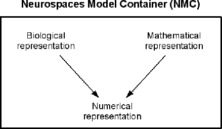
The Neurospaces Model Container (NMC) is the software component of NS that reads definitions of a biological model from source files, stores these data in memory, and translates them to the required mathematical entities.

In concordance with the CBI simulator functional architecture, the NMC is a stand-alone application that can be linked to GENESIS. The NMC deals purely with the biological entities and end-user concepts of a biophyscally realistic model rather than the mathematical equations that describe a model. It separates biological, physical and mathematical quantities of a simulation and ‘knows’ about biological entities such as neuronal circuits, single neurons, and their projections and connections. It also stores specific parameter values obtained from the literature as well as the actual parameter values employed during the simulation of a model. Functionally, the NMC is aware of neuronal morphology, membrane, and intracellular components such that the biological objects it contains rely hierarchically on their parents, children, and sibling’s parameters to infer a number of their own properties.

1.2 Neurospaces Studio

Neurospaces Studio (NSS) is a front-end to the NMC but is not a graphical editor or neuron construction kit. (External applications such as neuroConstruct, www.neuroconstruct.org, are more suited for that type of functionality.) Rather, NSS allows browsing, visualization, and validation of model parameters.

1.3 Heccer

Heccer (HEC) is a fast compartmental solver based on the hsolve functionality of the GENESIS simulator.

1.4 Simple Scheduler in Perl

The role of the Simple Scheduler in Perl (SSP) is to activate other stand-alone G-3 software components according to a configurable schedule. SSP ‘glues’ together these independent modules to ensure that they are activated correctly, such that they can work together on a single simulation.

2 Introduction to Neurospaces

This section contains general introductory comments about getting started with NS.

2.1 Neurospaces Model Descriptions

A Neurospaces Model Description File (NDF) is the format used to specify models, from those of intracellullar mechanisms to network models and morphologies. The file format is indicated by .ndf being appended to the name of a regular text file, e.g.

It is possible to convert neuron morphology files to NDF files using the command

(see section 5). A GENESIS script interface is currently under construction. This interface will allow GENESIS scripts to be run and execute the simulation, or simply convert the model specified by the GENESIS scripts to Neurospaces model descriptions.

A step-in example of consructing an NDF file can be found in section 3.

2.2 Overview of a NDF File

A NDF file contains four sections. These sections are not necessarily filled, but they must be present in the given order. A NDF file has the following general form (described in the following sections).

2.2.1 Header Section

The header must always be present and must always start with the interpreter sequence giving the system specific absolute path to the NMC executable:

This is followed by two declarations on separate lines. The first:

flags an appropriate major mode and keyword highlighting for Emacs and XEmacs editors¹ . The second declaration identifies the type of file, here:

2.2.2 Import Section

This section declares dependencies on other NDF files with the FILE keyword, e.g.

To simplify model development, NS allows construction of NDF files that define different components of a model. These files may be thought of as library files. To expedite model development, all NDF files can be shared by being imported into other NDF files.

The components declared in a NDF file can be either private to that NDF file, or public in that they can be shared with other NDF files. If a NDF file imports a second NDF file, only the public models of the imported file can be reused to build more complicated models in the importing file. This mechanism protects access to private models, while allowing reuse of the public models. The control on access is private to the imported NDF file. Thus, incomplete or unverified models should be contained within the private model section of a NDF file, whereas, finalized models should be constructed as public models. By this mechanism, NDF files containing public models, act as the library files that provide the basis of accelerated model development.

2.2.3 Private Model Section

These are models that are private to the NDF file that contains them. They may depend on imported public models of other files or be hard coded.

2.2.4 Public Model Section

These models are visible to the NDF files into which they are imported. Typically, for example, a neuron morphology would be located here. Public models may depend on private models or be hard coded.

2.2.5 Model Component Specification

Models are constructed from components defined by the occurence of predefined keywords and parameters known to NS, for example, SEGMENT for a somatic compartment, where the parameter DIA gives the diameter.

2.2.6 Miscellaneous

Units: NDF files define model components using SI Units.

Comment Syntax: Comments may be inserted into a NDF file in one of three ways:

• Unnested C comments of the normal form /* … */.
• Newline terminated C++ comments of the normal form //.
• Nested comments enclosed with {* and *}.

2.3 Validating a Model Description File

A NDF file can be validated by invoking:

This routine parses the file and tests for the coherence of the file syntax. A list of NS usage option flags can be obtained with:

3 A Simple Single Compartment Model

3.1 Introduction

As mentioned in section 1.1, in G-3 the definitions of biological models are read by the NMC, and stored in memory.

Because computational models in neuroscience often use a mixture of biological and mathematical representations, the NMC is internally aware of these categories and is able to translate both representations to the numerical formats required to run a simulation (see Fig. 1).

For example, HH-gates are mathematical constructs based on biological channels, such that the parameter values that define a gate are identical to their numerical representation.

However, dendritic segments are biological constructs with a number of mathematical properties. They have parameters with biological values as commonly reported in scientific papers, and must be converted to discrete compartments and their parameters with numerical values required for a numerical solver. This functionality is transparant to the user, and is explained in more detail in sections 3.4 and 3.5.

NOTE: From a user perspective, the NMC does not make a distinction between biological and mathematical representations of a model.

In the next paragraphs we outline the steps required to construct a NDF file that generates a single compartment model neuron. This model will generate action potentials via activation of the classical fast sodium and delayed rectifying potassium conductances as described by Hodgkin and Huxley (1952; J. Physiol. 117: 500).

The NDF files that generate this model can be found in the model library bundled with the NMC ² :

Following installation of the NS packages you should create a working directory for storing files used during model development, e.g.

Example commands, indicated below by $, were all issued after cd to that directory.

3.2 The HH Gates

The HH formalism is given by sodium and potassium conductances, where the total HH current is given by:

(1)

where

(2)

(3)

The behavior of the sodium conductance is determined by the kinetics of the m and h gates, and the behavior of the potassium conductance is determined by the kinetics of then gate. A gate can be in a permissive or non-permissive state, and an equation defines the gate kinetics as transitions between those two states. The state of the gate is the fraction of the population of potassium channels in a permissive state. It assumes a value between 0 and 1.

In a NDF file a gate is defined using the HH_GATE keyword. Inside a HH_GATE, the keyword GATE_KINETIC_FORWARD defines the parameters for transition from non-permissive to permissive states. The keyword GATE_KINETIC_BACKWARD defines the parameters for the reverse transition.

Since different simulators use different representations of the HH formalism, the formalism used by the NMC is a generalization of the HH formalism. For the sake of completeness we discuss these different representations, to define the relationship with the representation used by the NMC.

Commonly reported in the literature are steady state and time constant values, that are found using the formulae:

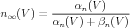(4)

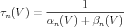(5)

And are related to α and β by the following equations:

(6)

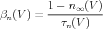(7)

For gate kinetics specification, the NMC uses an A-B based representation, that defines the following two functions:

(8)

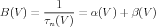(9)

and for converting back to the α-β form:

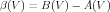(10)

(11)

The NMC Gate Description: The parameter names used to define a HH-like gate are based on the above A-B representation (a representation also used by the GENESIS 2 tabchan object). Its general form is:

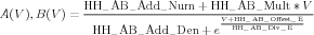(12)

In the NMC all these parameter names are prefixed with HH_, followed by a descriptor for the type of the gate representation, for example AB_ for parameters of the A - B based representation.

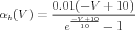
This equation corresponds to a general parameterized form for Hodgkin-Huxley type channel rate functions:

(13)

This is a generalization of the exponential, sigmoid, and linoid forms used by Hodgkin and Huxley (1952), with the variable y representing α(V ) or β(V ). It is used by the GENESIS 2 setupalpha command, which is implemented in the G-3 ns-sli module. This representation and its conversion from other rate expressions in other units is described in further detail in the document Conversion From Physiological to SI Units in GENESIS 3. The correspondence between the parameters A – F and those in Eq. 12, with their SI units, is given in the table:

There is one further parameter called the HH_AB_Factor_Flag parameter, having a default value of -1. If the value is set to +1, then it indicates that the denominator in Eq. 12 becomes a numerator or multiplier instead of a divisor, resulting in the equation:

(14)

This option is rarely used.

3.3 Simple Parameter Specification

For the sake of brevity, we discuss the definition of the n or activation gatecomplete explanation about activation, inactivation deactivation, deinactivation and list the full definition of all the gates. Then, we show how to use these gate definitions in the definition of a channel.

The HH formalism for the potassium channel assumes a sequence of four identical activation gates. In equation (3) the gate state of the potassium conductance is raised to the power of four.

The kinetics of the individual n gates of the potassium channel are determined by the functions α_h(V ) and β_h(V ) for which the definitions (in Physiological Units) are:

(15)

(16)

In the NMC, parameters are (name, value) tuples. Names are simple labels. Parameter values are defined using the PARAMETER token, which must occur within the scope of a PARAMETERS token. For example, to set HH_AB_Add_Num to -600.0 in the NDF file:

The model parameters of the forward rate of the n gate must be grouped together by using the PARAMETERS token. For example:

In the same way that the NMC recognizes public and private models, the NMC distinguishes between shared and private parameters of a model. Because some variables are shared between model components, they must be specifically declared, whereas this is not the case for private parameters.

Shared variables are declared within the component they are attached to by the INPUT and OUTPUT tokens, which must occur within the scope of BINDABLES. This allows shared variables of one component to be bound to those of another. The binding of variables is done with INPUT tokens within a block of BINDINGS. For example to declare Vm as an input to the n gate, and rate as an output of n gate:

To bind the Vm of the n gate to the Vm of the parent component, you write:

Collecting all these elements with a GATE_KINETIC_FORWARD token, the full definition of the forward rate becomes:

Similarly, for the backward rate we have:

The final two parameters required for complete specification of the n gate of the potassium channel, are POWER, indicating the power of the activation variable n, and state_init, giving the initial state of the gate. The reason why the initial state must be defined is because it is a solved variable³ . In GENESIS 2 the value of this parameter is implicitly set to the steady state value of the gate at the resting membrane potential. This approach is good for gates with small time constants. However, a more general approach is to initialize the state of the gates with values obtained after running the model.

The HH_GATE token is used to combine the forward and backward rate definitions, which is typically put in the public model section of an NDF file.

We are now in a position to combine the various definitions to give a complete description of the n gate specification of the HH potassium channel:

As explained above, an important feature of NS is that model cells can be constructed from a hierachy of fundamental building blocks or library files. The n gate that we have just defined is such a building block. It is defined as a public model in the NDF file, such that it is available to other NDF files for use in a channel definition. We choose to name the NDF file k_gate.ndf. The channel definition is then available for incorporation into a model soma (described in section 3.5).

For a more complete description of parameter and function specifications, see the multi-compartmental section (section 4).

NOTE: Functions can have regular parameters. For example, the Nernst equation description of the control of the potassium reversal potential by the intracellular calcium concentration:

NOTE: The definition of a model is always associated with a BINDABLES specification, while the use of a CHILD token is always associated with a BINDINGS specification.

3.4 Defining Channels

Every channel model consists of a number of gates. We have shown in the previous section how to define a single gate model based on the HH A-B formalism. This gate model was given the name k_gate_activation, and placed in the public model section of a NDF file with the name k_gate.ndf. It is then availabe for use in other model files.

To use the gate model, the public model section is imported with a FILE token and assigned to a namespace, here k_gate.

The ALIAS token, HH_K_n, makes the gate model available to the public models of the importing file:

After definition of the n gate, the potassium channel can be defined using the parameters G_MAX, E_REV, and CHANNEL_TYPE. G_MAX and E_REV define the conductance density and the channel reversal potential, respectively (see equation (1), page 19). The third parameter, CHANNEL_TYPE, distinguishes between channels with activation gates only (value ChannelAct), and channels with both activation and inactivation gates (value ChannelActInact). The CHILD token links the gate with the channel model:

3.5 Defining the Soma

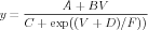
Historically, neuronal somas have been modeled as either cylinders or spheres. Cylindrical somata have both DIA and LENGTH parameters, spherical ones have their length undefined or set to zero.

The somatic compartment has membrane properties, for which we have to specify the appropriate parameters: specific resistance RM, specific capacitance CM and the reversal potential for the leak conductance ELEAK.

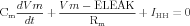(17)

where I_HH is defined by equation (1), and

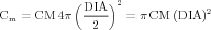(18)

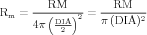(19)

NOTE: For the cylindrical representation, see section 4.

Just as the initial state of the gates was defined (see section 3.3), the initial state of the cell membrane must be defined, here using the Vm_init parameter.

To insert the previously defined sodium and potassium channel models into the membrane, they are assigned as children of the soma segment.

The channels provide a current that forms the input to the segment (I_HH), see equation (17)). The segment gives rise to the membrane potential, which is passed to the channels. The relationship between a channel and the membrane is formed by using shared variables that are declared using the BINDABLES token. The binding of the shared variables is done with INPUT tokens within a block of BINDINGS (see also section 3.3):

The complete NDF file with the definition of the soma is now given:

3.6 The Neuron Model

To complete the neuron model, the soma must be inserted into the model cell. This is done by importing the soma definition into the private model section of a NDF file. The ALIAS token makes the definition available to the public model section (see also section 3.4). The model cell is then created using a CELL token, and the soma segment is assigned as a child inside this token:

3.7 Running a Simulation

A simulation is started using the ssp command. This reads a SSP configuration file that controls the simulation, including the stimulation protocol and simulation output. For expediency, the ssp command has builtin configurations for running different types of simulation⁴ . The --cell option selects the builtin configuration for running a single neuron model. The required argument is a reference to the NDF file that contains the model to be simulated. First, an environment variable is set to instruct the NMC where to find this file:

We can then run the model:

The duration of the simulation and its temporal resolution are given respectively by the --time and --time-step options. Both options take an amount of time specified in seconds. The default time step is 20 μs (2e-5 s in SI units), while the default simulation time is 50 ms.

By default, the output of a simulation using the --cell configuration is the membrane potential at the soma. It is stored in a file that takes its name from the NDF argument passed to SSP. For our single compartment model, this is output/hh_neuron. Additional command line options are available that overwrite specific --cell defaults, and define other stimuli and outputs. For example, the --inject-magnitude option specifies the magnitude of somatic current injection. The time course of the current injection is given by the --inject-delay and --inject-duration options. The --parameters option will allow initialization of other input parameters.

For example to inject a current into the soma with magnitude 2 nA for the duration of the simulation:

To run the same simulation using the --parameters option:

Here, the --parameters option assigns a value to a model parameter using a syntax specific for the NMC. Note that the use of single quotes is required to protect the argument string from being interpreted as an output redirection command to a file with a peculiar name.

Specific outputs are defined with the --output option. The default filename for this option is inferred from the NDF filename, and this file is placed in the directory ./output/, which is created if it does not exist. For example, to store the somatic membrane potential, the command:

will generate an output file named output/hh_neuron.out. By convention, the default output filename has an .out extension. The output filename can be changed using the --outputclass-filename option:implement.

NOTE: The ./hh_neuron/ directory is created automatically.

Synaptic stimulation: The model defined in the previous sections does not contain synapses, and can only be stimulated by current injection. Here, we first show how to add synapses to the model, then how to activate the them. Synaptic activation can be done in two ways. (1) Set the firing frequency of spontaneous activity. This frequency is a parameter of the synaptic channel, and the weight of the activated synapse is always one. This type of activation is commonly used to simulated an in vivo condition. (2) Attach a series of precalculated synaptic event times stored in a file to the synaptic channel.

add afferents to the model

When using builtin configurations, the names of the simulation schedule and the output file can be defined using the command line flags --set-name and --set-outputclass-filename, respectively.

3.8 Initialization of Simulation Variables

• --dump-variables
• --undump-variables

4 A Multicompartmental Model

4.1 Morphology

Discuss morphology2ndf here.

4.2 Symbolic Parameter Specifications

Values are either constant, point to a parameter of another symbol, or have a function value. As an example:

Here, the DIAMETER parameter has a constant value, the LENGTH parameter is inherited from the parent component (the ’..’ notation is a reference to the parent symbol⁵ ), and SEED has a value defined by the function SERIAL().

4.3 Running the model

5 The Morphology Convertor

A .ndf file can be generated from a .swc (or a GENESIS .p) morphology file by running:

NOTE: The redirection arrow (>) in the above statement. A list of the optional conversion parameters is obtained with:

As mentioned above, neuron morphology files can be converted to NDF files using the command morphology2ndf. Under normal circumstances this command is called and configured automatically by the simulator. The configuration of this command is done via a configuration file. If a configuration file is not given as a flagged argument in the command line, e.g.

a default configuration file based on the De Schutter & Bower 1994 Purkinje neuron paper (J. Neurophysiol. 71: 375) is used. The contents of this file (which is currently being used by regression tests) is obtained with:

which returns:

NOTE: In the configuration file, the value indicator (http://www.yaml.org/refcard.html), a single colon :, indicates an unordered list (see in above example following aliasses) and the nested series indicator, a dash (-), indicates an ordered list (see in above example following parameter_2_prototype). Importantly, the configuration file is white space sensitive and tabulators are not allowed for spacing.

The aliasses of the configuration file:

are inserted into the scope of the IMPORT token in the NDF file during the command:

The default entries for the key parameter_2_prototype enumerate the prototype(s) in order of increasing diameter. Thus, (i) spiny dendrites include all compartments < 3.18e^-6, (ii) 3.18e^-6 < thick dendrites < 7.71e^-6, (iii) 7.71e^-6 < main dendrite < 2.8e^-5, and (iv) 2.8e^-5 < soma < 1.

An alternative way to specify prototypes in the configuration file is with the flags defined for a .swc morphology file that tag the location of different neuronal compartments:

The De Schutter and Bower (1994) Purkinje cell model can not be exactly reproduced this way from its original morphology file. This is due to a small difference between the distribution of the active channels in the model vs. the output of morphology2ndf. To solve this problem, a second key (name_2_prototype) can be optionally included into the configuration file. It defines a mapping of names to prototypes as opposed to parameters to prototypes. The key behaves essentially the same asparameter_2_prototype, but instead of looking at a parameter value such as dia or tag, it looks at the names of the segments in the morphology file. When the name matches, this key takes higher priority than the parameter_2_prototype key. Thus a regular mapping of the morphology to an active model is given using the parameter_2_prototype key with an additional number of hardcoded exceptions given by the key name_2_prototype’, such that morphology2ndf can produce an exact match with the Purkinje cell model.

NOTE: The inline comments included in the above examples and indicated by // are inserted here for clarification but are not permitted in the actual configuration file. As mentioned above, the command line arguments to morphology2ndf can be used to overwrite default configuration values before any conversion takes place, e.g. to change the shrinkage factor:

This will replace the default shrinkage correction factor of 1 with the given value (1.1111) in my.ndf.

6 Appendix

6.1 Neurospaces Parameter Definitions

The following <name,label> tuples are recognized by Neurospaces:

6.1.1 cached_connection

DELAY: Connection delay.
PRE: Connection presynaptic serial identifier.
POST: Connection postsynaptic serial identifier.
WEIGHT: Connection weight.

6.1.2 channel

CHANNEL_TYPE: Defines the following channel types:
ChannelActInact: Channel with activation and inactivation gates.
ChannelAct: Channel with activation gate.
ChannelActConc: Channel with activation and concentration gates.
Ek: Channel reversal potential.
G_MAX: Maximal conductance density when all channels are in the open state.
Gk: Actual channel conductance, normally a solved variable.
Ik: Actual channel current, normally a solved variable.

6.1.3 concentration_gate_kinetic

BASE: Basal level, A in De Schuter & Bower, 1994.
TAU: Time constant, B in De Schuter & Bower, 1994.

6.1.4 connection

DELAY: Connection delay.
PRE: Connection presynaptic serial identifier.
POST: Connection postsynaptic serial identifier.
WEIGHT: Connection weight.

6.1.5 connection_symbol

DELAY: Connection delay.
PRE: Connection presynaptic serial identifier.
POST: Connection postsynaptic serial identifier.
WEIGHT: Connection weight.

6.1.6 contour_point

THICKNESS: Thickness of the slice originating the contour.

6.1.7 equation

TAU1: First time constant.
TAU2: Second time constant.

6.1.8 fiber

RATE: Average firing frequence, bind it to the threshold of a spikegenerator.
REFRACTORY: Absolute refractory period.

6.1.9 gate_kinetic

DeNominatorOffset: 4: Nominator or denominator offset.
MembraneDependence: 2: Multiplier membrane dependence, 0.0 for no dependence.
MembraneOffset: 5: Membrane offset.
Multiplier: 1: Multiplier.
Nominator: 3: Choose between nominator or denominator, 1 means nominator, -1 denominator.
TauDenormalizer: 6: Denormalized time constant.

6.1.10 h_h_gate

POWER: Gate power.
state: Current state, normally a solved variable.
state_init: Initial value, commonly forward over backward steady states.

6.1.11 pool

BASE: Basal concentration level.
BETA: Fixed beta (use the FIXED function to avoid scaling).
DIA: Concentration pool diameter, normally the same as the segment diameter.
LENGTH: Concentration pool length, normally the same as the segment length.
TAU: Concentration pool time constant.
THICK: Concentration pool thickness.
VAL: Ion valency.
concen: Actual concentration value, normally a solved variable.
concen_init: Initial concentration level.

6.1.12 population

EXTENT_X, EXTENT_Y, EXTENT_Z: Coordinate of the last cell minus coordinate of the first cell.

6.1.13 projection

SOURCE: Source population.
TARGET: Target population.

6.1.14 randomvalue

LENGTH: Length, for visualization purposes only.
MAXIMUM: Maximum value the random variable can take
MINIMUM: Minimum value the random variable can take.

6.1.15 segment

CM: Specific capacitance of this segment.
RA: Specific axial resistance of this segment.
RM: Specific membrane resistance of this segment.
SOMATOPETAL_DISTANCE: Somatopetal distance of the segment.
TAU: Time constant of the segment, CM*RM.
Vm: Membrane potential, normally a solved variable.
Vm_init: Initial membrane potential.

6.1.16 segmenter

DIA: Segment diameter.
LENGTH: Segment length (calculated automatically if not set).
PARENT: Parent segment, somatopetal.
SURFACE: Surface of the segment (calculated automatically if not set, you can set it to add spine surface).
TOTALSURFACE: Total surface of all segments in the segmenter (calculated automatically).
rel_X, rel_X, rel_X: Spatial extent of the segment in the X, Y, and Z directions.

6.1.17 symbol

ROTATE_ANGLE: Relative coordinate transformation.
ROTATE_AXIS_X, ROTATE_AXIS_Y, ROTATE_AXIS_Z: Relative coordinate transformations.
ROTATE_CENTER_X, ROTATE_CENTER_Y, ROTATE_CENTER_Z: Relative coordinate transformations.
X, Y, Z: Coordinated relative to parent.

6.2 Neurospaces Algorithm Instances

The following ?? are rocognized by Neurospaces.

6.2.1 connectionchecker

PROJECTION_NAME: Name of projection to check.

6.2.2 grid3d

PROTOTYPE: Reference to the biological component to layout in a grid.
X_COUNT, Y_COUNT, Z_COUNT: Number of instances to create in the X, Y, and Z directions.
X_DISTANCE, Y_DISTANCE, Z_DISTANCE: Separation between two instances in the X, Y, and Z directions.

6.2.3 inserter

HEIGHTS_PARAMETER_FILENAME: Filename with distances to base and prototype references.
INSERTION_FREQUENCY: Probability of insertion.
NAME_SELECTOR: Name matcher, selects segment candidates for receiving additional components by name.

6.2.4 projectionrandomized

DELAY_TYPE: Fixed delay (FIXED_DELAY) or radial (VELOCITY).
DESTINATION_TYPE: ‘box’ or ‘ellipse’.
DESTINATION_X1, DESTINATION_Y1, DESTINATION_Z1: Destination box, X, Y, Z coordinate boundary bottom left front.
DESTINATION_X2, DESTINATION_Y2, DESTINATION_Z2: Destination box, X, Y, Z coordinate boundary top right back.
FIXED_DELAY: Fxed delay.
PRE: Pre synaptic name selector.
POST: Post synaptic name selector.
PROBABILITY: Connection probability.
PROJECTION_NAME: Name of projection to check.
RANDOMSEED: Randomization seed.
SOURCE_TYPE: ‘box’ or ‘ellipse’.
SOURCE_X1, SOURCE_Y1, SOURCE_Z1: Source box, X, Y, Z coordinate boundary bottom left front.
SOURCE_X2, SOURCE_Y2, SOURCE_Z2: Source box, X, Y, Z coordinate boundary top right back.
VELOCITY: Action propagation velocity.
WEIGHT: Fixed weight.

6.2.5 randomize

LOWER_BOUND: Lower bound for the randomized parameter values.
PARAMETER_NAME: Parameter to randomize.
RANDOMSEED: Randomization seed.
SYMBOL_NAME: Component to randomize a parameter for.
TARGET_NAME: Name of prototype target to randomize.
UPPER_BOUND: Upper bound for the randomized parameter values.

6.2.6 replacer

NAME_SELECTOR: Name matcher, selects segment candidates for replacement by name.
PROTOTYPE: Reference to the biological component to layout in a grid.

6.2.7 spines

DIA_MAX: Random spines maximal dendritic diameter for segment.
DIA_MIN: Random spines minimal dendritic diameter for segment.
NAME_SELECTOR: Name matcher, selects segment candidates for receiving spines, if not given all segments match.
PROTOTYPE: Reference to the spine definition.
SPINE_DENSITY: Spine density, in spines per μm.
SPINE_FREQUENCY: Spine insertion probability.

7 References

1 Cornelis, H. (2007) CBI simulator functional architecture. Unpublished Technical Report.
   Found at: www.neurospaces.sourceforge.net/cbi.png.
2 Cornelis, H. (2003) Neurospaces software design. Unpublished Technical Report.

References